Open-circuit test

The open-circuit test, or "no-load test", is one of the methods used in electrical engineering to determine the no-load impedance in the excitation branch of a transformer.

Method

The secondary of the transformer is left open-circuited. A wattmeter is connected to the primary. An ammeter is connected in series with the primary winding. A voltmeter is optional since the applied voltage is the same as the voltmeter reading. Rated voltage is applied at primary.

If the applied voltage is normal voltage then normal flux will be set up. Since iron loss is a function of applied voltage, normal iron loss will occur. Hence the iron loss is maximum at rated voltage. This maximum iron loss is measured using the wattmeter. Since the impedance of the series winding of the transformer is very small compared to that of the excitation branch, all of the input voltage is dropped across the excitation branch. Thus the wattmeter measures only the iron loss. This test only measures the combined iron losses consisting of the hysteresis loss and the eddy current loss. Although the hysteresis loss is less than the eddy current loss, it is not negligible. The two losses can be separated by driving the transformer from a variable frequency source since the hysteresis loss varies linearly with supply frequency and the eddy current loss varies with the square.

Since the secondary of the transformer is open, the primary draws only no-load current, which will have some copper loss. This no-load current is very small and because the copper loss in the primary is proportional to the square of this current, it is negligible. There is no copper loss in the secondary because there is no secondary current.

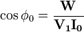
Current, voltage and power are measured at the primary winding to ascertain the admittance and power-factor angle.

Another method of determining the series impedance of a real transformer is the short circuit test.

Calculations

The current $\mathbf{I_0}$ is very small.

If $\mathbf{W}$ is the wattmeter reading then,

$\mathbf{W} = \mathbf{V_1} \mathbf{I_0} \cos \phi_0$

That equation can be rewritten as,

$\cos \phi_0 = \frac {\mathbf{W}} {\mathbf{V_1} \mathbf{I_0}}$

Thus,

$\mathbf{I_m} = \mathbf{I_0} \sin \phi_0$

$\mathbf{I_w} = \mathbf{I_0} \cos \phi_0$

Impedance

By using the above equations, $\mathbf{X_0}$ and $\mathbf{R_0}$ can be calculated as,

$\mathbf{X_0} = \frac {\mathbf{V_1}} {\mathbf{I_m}}$

$\mathbf{R_0} = \frac {\mathbf{V_1}} {\mathbf{I_w}}$

Thus,

$\mathbf{Z_0} = \sqrt {\mathbf{R_0}^2 +\mathbf{X_0}^2}$

or

$\mathbf{Z_0} = \mathbf{R_0} + \mathbf{j} \mathbf{X_0}$

Admittance

The admittance is the inverse of impedance. Therefore,

$\mathbf{Y_0} = \frac {1} {\mathbf{Z_0}}$

The conductance $\mathbf{G_0}$ can be calculated as,

$\mathbf{G_0} = \frac {\mathbf{W}} {\mathbf{V_1}^2}$

Hence the susceptance,

$\mathbf{B_0} = \sqrt {\mathbf{Y_0}^2 -\mathbf{G_0}^2}$

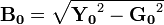
or

$\mathbf{Y_0} = \mathbf{G_0} + \mathbf{j} \mathbf{B_0}$

Here,

$\mathbf{W}$ is the wattmeter reading

$\mathbf{V_1}$ is the applied rated voltage

$\mathbf{I_0}$ is the no-load current

$\mathbf{I_m}$ is the magnetizing component of no-load current

$\mathbf{I_w}$ is the core loss component of no-load current

$\mathbf{Z_0}$ is the exciting impedance

$\mathbf{Y_0}$ is the exciting admittance

References

• Kosow (2007). Electric Machinery and Transformers. Pearson Education India. 
• Smarajit Ghosh (2004). Fundamentals of Electrical and Electronics Engineering. PHI Learning Pvt. Ltd. 
• Wildi, Wildi Theodore (2007). Electrical Machines , Drives And Power Systems, 6th edtn. Pearson. 

See also

• Short-circuit test
• Thévenin's theorem
• Blocked rotor test
• Circle diagram